
The concept of the Limits and Continuity is one of the most crucial things to understand in order to prepare for calculus.
Who invented calculus?
Gottfried Leibnitz is a famous German philosopher and mathematician and he was a contemporary of Isaac Newton. These two gentlemen are the founding fathers of Calculus and they did most of their work in 1600s. We still use the Leibniz notation of dy/dx for most purposes.
Limit
A limit is a number that a function approaches as the independent variable of the function approaches a given value. For example, given the function f (x) = 3x , you could say, “The limit of f (x) as x approaches 2 is 6 .” Symbolically, this is written  f (x) = 6 .
Continuity
Continuity is another far-reaching concept in calculus. A function can either be continuous or discontinuous. One easy way to test for the continuity of a function is to see whether the graph of a function can be traced with a pen without lifting the pen from the paper. For the math that we are doing in precalculus and calculus, a conceptual definition of continuity like this one is probably sufficient, but for higher math, a more technical definition is needed. Using limits, we’ll learn a better and far more precise way of defining continuity as well. With an understanding of the concepts of limits and continuity, you are ready for calculus.
The Idea of Limits of Functions
We all know about functions, A function is a rule that assigns to each element xfrom a set known as the “domain” a single element yfrom a set known as the “range“. For example, the function y = x 2 + 2 assigns the value y = 3 to x = 1 , y = 6to x = 2 , and y = 11 to x = 3. Using this function, we can generate a set of ordered pairs of (x, y) including (1, 3),(2, 6), and (3, 11).
The idea behind limits is to analyze what the function is “approaching” when x “approaches” a specific value. To start getting used to this idea, let’s turn to this graph:
When x approaches the value “a” in the x axis, the function f(x) approaches “L” in the y axis. In this graph I drawed a big pink hole at the point (a,L). I do this because we don’t necessarily know the value of function f at x=a.
Let’s turn to the graph of a function whose expression we know:
This is the function f(x)=x2. Let’s focus on the point (1,1). We can see from the graph that when x approaches 1, the function f(x) approaches 1. When this happens, we say that:

This is read “the limit as x approaches 1 of x squared equals 1”.
Why Limits and Continuity is Useful
You might ask what this is useful for. Very good question. Why would you need to know what the function is approaching? You already know the function equals 1 when x equals 1, right?
Well, the point is that sometimes we don’t care what the function is at x=1.
As an example of this, let’s consider the following function:

Don’t let this notation intimidate you! This only means that this function equals x2 when x is anything other than 1, and equals 0 when x equals 1. This function is the same as the one we saw before, but in this case it has a “hole” at x=1. Let’s see what the graph looks like:

What does the function approach when x approaches 1? It also approaches 1, right? It doesn’t matter that the function is other than 1 at that point! So,

In calculus, the most useful limits are like this one. The value of the function at the specific point we care about is not defined, like 0/0 (which is complete junk), or useless, like zero or infinite.
The Idea of Continuous Functions
Limits and continuity are often covered in the same chapter of textbooks. This is because they are very related. The basic idea of continuity is very simple, and the “formal” definition uses limits.
Basically, we say a function is continuous when you can graph it without lifting your pencil from the paper. Here’s an example of what a continuous function looks like:
There is a precise mathematical definition of continuity that uses limits. Intuitively, this definition says that small changes in the input of the function result in small changes in the output.
If you are confused by that, ignore it! You don’t need to learn all at once. The most important is to recognize a continuous function when you see it.
Now, what would a discontinuous function look like? A function essentially is discontinuous when it has any “gap”. For example:
There are three types of discontinuities:
Discontinuity 1: Asymptotic Discontinuities
Asymptotes occur when a function approaches infinity at a specific value of x or y. If a function has values on both sides of an asymptote, then it cannot be connected, so it must have a discontinuity at the asymptote. We look for asymptotes at points where the denominator is zero because: when the denominator gets close to zero and becomes very small, it makes the value of the function very large. For example, if we look at the fraction ![]() , i.e. divide 5 by 0.1, we get that it equals 50. If we make the denominator smaller, the value of the fraction gets larger:
, i.e. divide 5 by 0.1, we get that it equals 50. If we make the denominator smaller, the value of the fraction gets larger: ![]() = 500, = 500000. This tells us that the closer to zero that the denominator is, the larger the value of the fraction. In other words, we’ve demonstrated
= 500, = 500000. This tells us that the closer to zero that the denominator is, the larger the value of the fraction. In other words, we’ve demonstrated
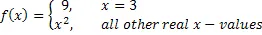
Discontinuity 2: Point Discontinuities
Point discontinuities occur when a function is defined specifically for an isolated x-value. However, this does not guarantee a point discontinuity. For example, if we change our function slightly to it becomes continuous. This is because we have defined the value of the function at f(3) precisely to be the value of the function 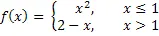 at x = 3. In this case, we did not define the value at = 3 to be different from what it would be if the function were
 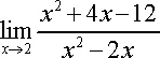 . Then there is no discontinuity. Compared to our last function with a point discontinuity, we moved the point back up to the function to “plug” up the hole, and it is now continuous. Always remember, if a function is defined like this, to check if the isolated point is a point discontinuity or just a trick.
Discontinuity 3: Jump Discontinuities
Jump discontinuities are also called simple discontinuities, or continuities of the first kind.
Just as we can define a function at a specific point, we can also define a function in specific regions. Consider the function Let’s work on an example
Estimate the value of the following limit
Solution
Notice that I did say estimate the value of the limit. Again, we are not going to directly compute limits in this section. The point of this section is to give us a better idea of how limits work and what they can tell us about the function.
So, with that in mind we are going to work this in pretty much the same way that we did in the last section. We will choose values of x that get closer and closer to x=2 and plug these values into the function. Doing this gives the following table of values.
| x | f(x) | x | f(x) |
| 2.5 | 3.4 | 1.5 | 5.0 |
| 2.1 | 3.857142857 | 1.9 | 4.157894737 |
| 2.01 | 3.985074627 | 1.99 | 4.015075377 |
| 2.001 | 3.998500750 | 1.999 | 4.001500750 |
| 2.0001 | 3.999850007 | 1.9999 | 4.000150008 |
| 2.00001 | 3.999985000 | 1.99999 | 4.000015000 |
Note that we made sure and picked values of x that were on both sides of and that we moved in very close to to make sure that any trends that we might be seeing are in fact correct. Also notice that we can’t actually plug in into the function as this would give us a division by zero error. This is not a problem since the limit doesn’t care what is happening at the point in question.
From this table it appears that the function is going to 4 as x approaches 2, so
= 4
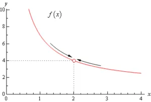
Let’s think a little bit more about what’s going on here. Let’s graph the function from the last example. The graph of the function in the range of x’s that were interested in is shown below. First, notice that there is a rather large open dot at . This is there to remind us that the function (and hence the graph) doesn’t exist at .
As we were plugging in values of x into the function we are in effect moving along the graph in towards the point as . This is shown in the graph by the two arrows on the graph that are moving in towards the point.
When we are computing limits the question that we are really asking is what y value is our graph approaching as we move in towards on our graph. We are NOT asking what y value the graph takes at the point in question. In other words, we are asking what the graph is doing around the point . In our case we can see that as x moves in towards 2 (from both sides) the function is approaching even though the function itself doesn’t even exist at . Therefore we can say that the limit is in fact 4.
So what have we learned about limits? Limits are asking what the function is doing around and are not concerned with what the function is actually doing at . This is a good thing as many of the functions that we’ll be looking at won’t even exist at as we saw in our last example.